Poisson equation using Python for source term specification

Elliptic/square_1x1_SteadyStateDiffusion_Python/square_1e3_poisson_sin_x_sin_y.prj

Poisson Equation

The Poisson equation is:

$$ \begin{equation} \- k\\;\Delta p = Q \quad \text{in }\Omega \end{equation}$$

w.r.t boundary conditions

$$ \eqalign{ p(x) = g_D(x) &\quad \text{on }\Gamma_D,\cr k\\;{\partial p(x) \over \partial n} = g_N(x) &\quad \text{on }\Gamma_N, }$$

where $p$ could be the pressure, the subscripts $D$ and $N$ denote the Dirichlet- and Neumann-type boundary conditions, $n$ is the normal vector pointing outside of $\Omega$, and $\Gamma = \Gamma_D \cup \Gamma_N$ and $\Gamma_D \cap \Gamma_N = \emptyset$.

Problem specification and analytical solution

We solve the Poisson equation on a square domain $\Omega = [0\times 1]^2$ with $k = 1$ w.r.t. the specific boundary conditions:

$$ \eqalign{ p(x,y) = 1 &\quad \text{on } (x=0,y=0) \subset \Gamma_D,\cr p(x,y) = 1 &\quad \text{on } (x=0,y=1) \subset \Gamma_D,\cr p(x,y) = 1 &\quad \text{on } (x=1,y=0) \subset \Gamma_D,\cr p(x,y) = 1 &\quad \text{on } (x=1,y=1) \subset \Gamma_D,\cr }$$

and the source term is

$$ Q(x,y) = a^2 \sin\left(ax - \frac{\pi}{2}\right) \sin\left(by - \frac{\pi}{2}\right) +b^2 \sin\left(ax - \frac{\pi}{2}\right) \sin\left(by - \frac{\pi}{2}\right) $$

The analytical solution of (1) is

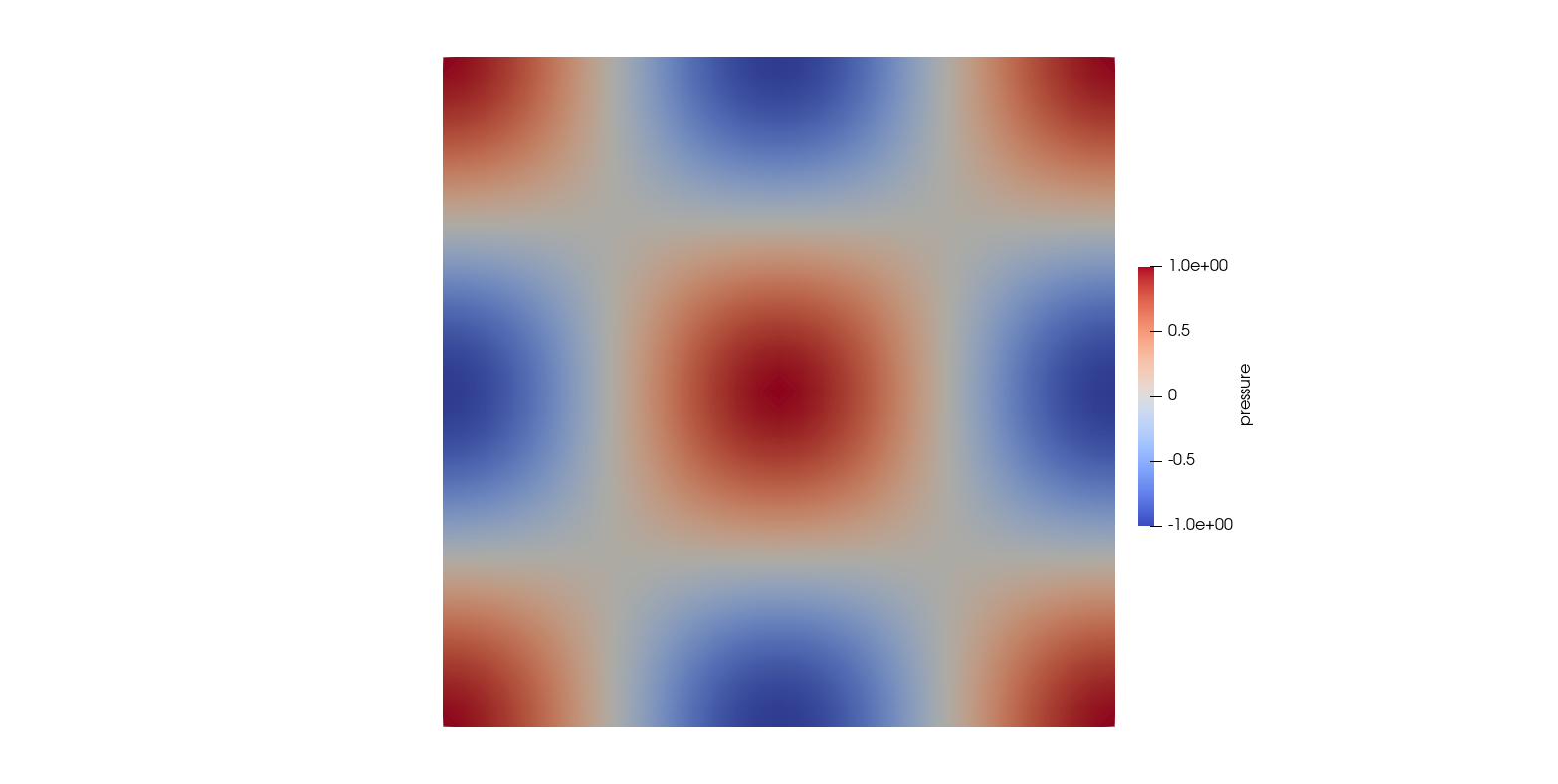
$$ p(x,y) = \sin\left(ax - \frac{\pi}{2}\right) \sin\left(by - \frac{\pi}{2}\right). $$

Since

$$ \frac{\partial^2 p}{\partial x} (x,y) = - a^2 \sin\left(ax - \frac{\pi}{2}\right) \sin\left(by - \frac{\pi}{2}\right) $$

and

$$ \frac{\partial^2 p}{\partial y} (x,y) = - b^2 \sin\left(ax - \frac{\pi}{2}\right) \sin\left(by - \frac{\pi}{2}\right) $$

it yields

$$ \Delta p(x,y) = - a^2 \sin\left(ax - \frac{\pi}{2}\right) \sin\left(by - \frac{\pi}{2}\right) - b^2 \sin\left(ax - \frac{\pi}{2}\right) \sin\left(by - \frac{\pi}{2}\right) $$

and

$$ Q = - \Delta p(x,y) = a^2 \sin\left(ax - \frac{\pi}{2}\right) \sin\left(by - \frac{\pi}{2}\right) + b^2 \sin\left(ax - \frac{\pi}{2}\right) \sin\left(by - \frac{\pi}{2}\right). $$

Input files

The project file is square_1e3_poisson_sin_x_sin_y.prj. It describes the process to be solved and the related process variable together with their initial, boundary conditions and source terms. The definition of the source term $Q$ is in a Python script. The script for setting the source terms is referenced in the project file as follows:

<python_script>sin_x_sin_y_source_term.py</python_script>

In the source term description

<source_term>
    <mesh>square_1x1_quad_1e3_entire_domain</mesh>
    <type>Python</type>
    <source_term_object>sinx_siny_source_term</source_term_object>
</source_term>

the domain is specified by the mesh-tag. The function $Q$ is defined by the Python object sinx_sinx_source_term that is created in the last line of the Python script:

try:
    import ogs.callbacks as OpenGeoSys
except ModuleNotFoundError:
    import OpenGeoSys

from math import pi, sin

a = 2.0*pi
b = 2.0*pi

def solution(x, y):
    return - sin(a*x-pi/2.0) * sin(b*y-pi/2.0)

# - laplace(solution) = source term
def laplace_solution(x, y):
    return a*a * sin(a*x-pi/2.0) * sin(b*y-pi/2.0) + b*b * sin(a*x-pi/2.0) * sin(b*y-pi/2.0)

# source term for the benchmark
class SinXSinYSourceTerm(OpenGeoSys.SourceTerm):
    def getFlux(self, t, coords, primary_vars):
        x, y, z = coords
        value = laplace_solution(x,y)
        Jac = [ 0.0 ]
        return (value, Jac)

# instantiate source term object referenced in OpenGeoSys' prj file
sinx_siny_source_term = SinXSinYSourceTerm()

Running simulation

To start the simulation (after successful compilation) run:

ogs square_1e3_poisson_sin_x_sin_y.prj

It will produce some output and write the computed result into the square_1e3_volumetricsourceterm_pcs_0_ts_1_t_1.000000.vtu, which can be directly visualized and analysed in ParaView for example.

The output on the console will be similar to the following on:

info: This is OpenGeoSys-6 version 6.1.0-1132-g00a6062a2.
info: OGS started on 2018-10-10 09:22:17+0200.

info: ConstantParameter: K
info: ConstantParameter: p0
info: ConstantParameter: pressure_edge_points
info: Initialize processes.
createPythonSourceTerm
info: Solve processes.
info: [time] Output of timestep 0 took 0.000695229 s.
info: === Time stepping at step #1 and time 1 with step size 1
info: [time] Assembly took 0.0100119 s.
info: [time] Applying Dirichlet BCs took 0.000133991 s.
info: ------------------------------------------------------------------
info: *** Eigen solver computation
info: -> solve with CG (precon DIAGONAL)
info:    iteration: 81/10000
info:    residual: 5.974447e-17

info: ------------------------------------------------------------------
info: [time] Linear solver took 0.00145817 s.
info: [time] Iteration #1 took 0.0116439 s.
info: [time] Solving process #0 took 0.011662 s in time step #1
info: [time] Time step #1 took 0.0116858 s.
info: [time] Output of timestep 1 took 0.000671864 s.
info: The whole computation of the time stepping took 1 steps, in which
         the accepted steps are 1, and the rejected steps are 0.

info: [time] Execution took 0.0370049 s.
info: OGS terminated on 2018-10-10 09:22:17+020

Results and evaluation

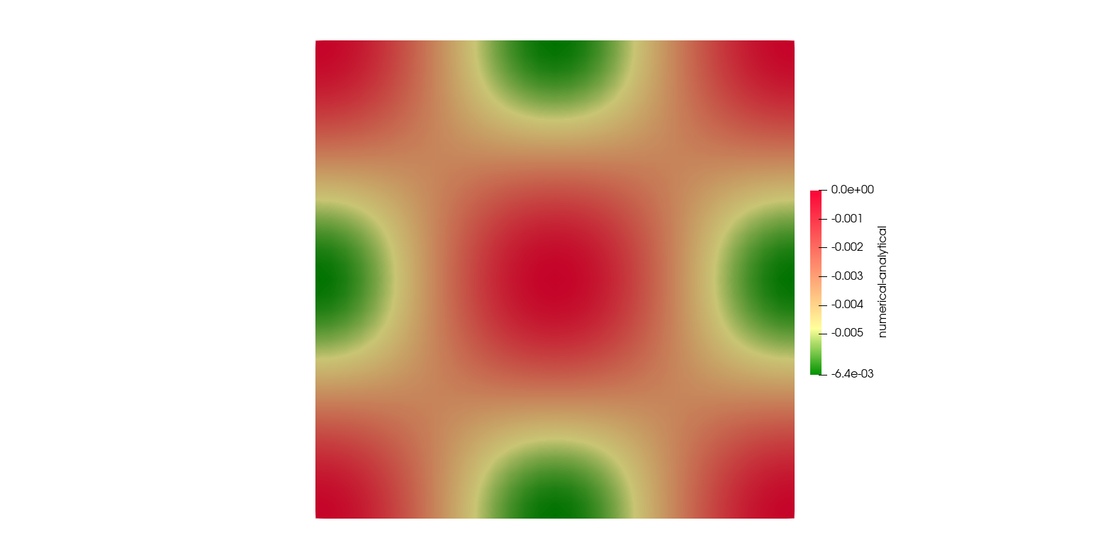
Comparison of the numerical and analytical solutions

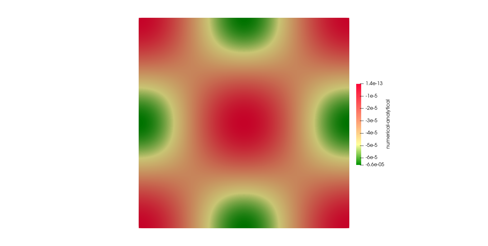
The above picture shows the numerical result. The solution conforms in the edges to the prescribed boundary conditions.

Since a coarse mesh ($32 \times 32$ elements) is used for the simulation the difference between the numerical and the analytical solution is relatively large.

Comparison for higher resolution mesh ($316 \times 316$ elements)

The difference between the numerical and the analytical solution is much smaller than in the coarse mesh case.

This article was written by Tom Fischer. If you are missing something or you find an error please let us know.
Generated with Hugo 0.122.0 in CI job 520198 | Last revision: July 8, 2024
Commit: [LD] Changed shape function its gradient names 6c1906cd | Edit this page on