Injection and Production in 1D Linear Poroelastic Medium with the Staggered Scheme

HydroMechanics/StaggeredScheme/InjectionProduction1D/InjectionProduction1D.prj

Injection and Production in 1D Linear Poroelastic Medium

This benchmark simulates a soil column with fluid injection at the bottom and a production well at the top. It is taken from Kim [1], in detail it coincides with one of his examples (case 2, coupling strength $τ = 1.21$ ). A brief description of the used staggered scheme follows at the end.

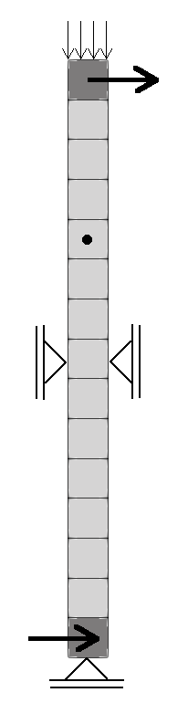
Simulation model with fluid source, sink, observation point and boundary conditions

The fluid enters and leaves only via the source and sink in the domain, there is no flow across the boundaries. The displacements at the bottom are fixed, whereas there is a vertical traction applied on top. Originally the problem is one-dimensional, for simulation with OpenGeoSys it is created in two dimensions with corresponding boundary conditions. All parameters are concluded in the following tables.

Material Properties
Property	Value	Unit
Fluid density	$10^{3}$	kg/m $^{3}$
Viscosity	$10^{- 3}$	Pa $\cdot$ s
Fluid compressibility	$27.5 \cdot 10^{- 9}$	Pa $^{- 1}$
Porosity	$0.3$	-
Permeability	$493.5 \cdot 10^{- 16}$	m $^{2}$
Young’s modulus (bulk)	$300 \cdot 10^{6}$	Pa
Poisson ratio (bulk)	$0$	-
Biot coefficient	$1.0$	-
Solid density	$3 \cdot 10^{3}$	kg/m $^{3}$
Solid compressibility	$0$	Pa $^{- 1}$

Dimensions and Discretization
Property	Value	Unit
Height ( $y$ )	$150$	m
Width ( $x$ )	$10$	m
Finite Elements	$15$ Taylor-Hood quadrilateral elements	10 m $\times$ 10 m
Time step	$86.4 \cdot 10^{3}$	s

Sources/Sinks, Initial and Boundary Conditions
	Hydraulic	Mechanical
injection over area $10$ m $\times 10$ m	$+ 1.16 \cdot 10^{- 4}$ kg/(m $^{3}$ s)	-
production over area $10$ m $\times 10$ m	$- 1.16 \cdot 10^{- 4}$ kg/(m $^{3}$ s)	-
top	no flow	$σ_{y y} = - 2.125 \cdot 10^{6}$ Pa
left	no flow	$u_{x} = 0$
right	no flow	$u_{x} = 0$
bottom	no flow	$u_{y} = 0$
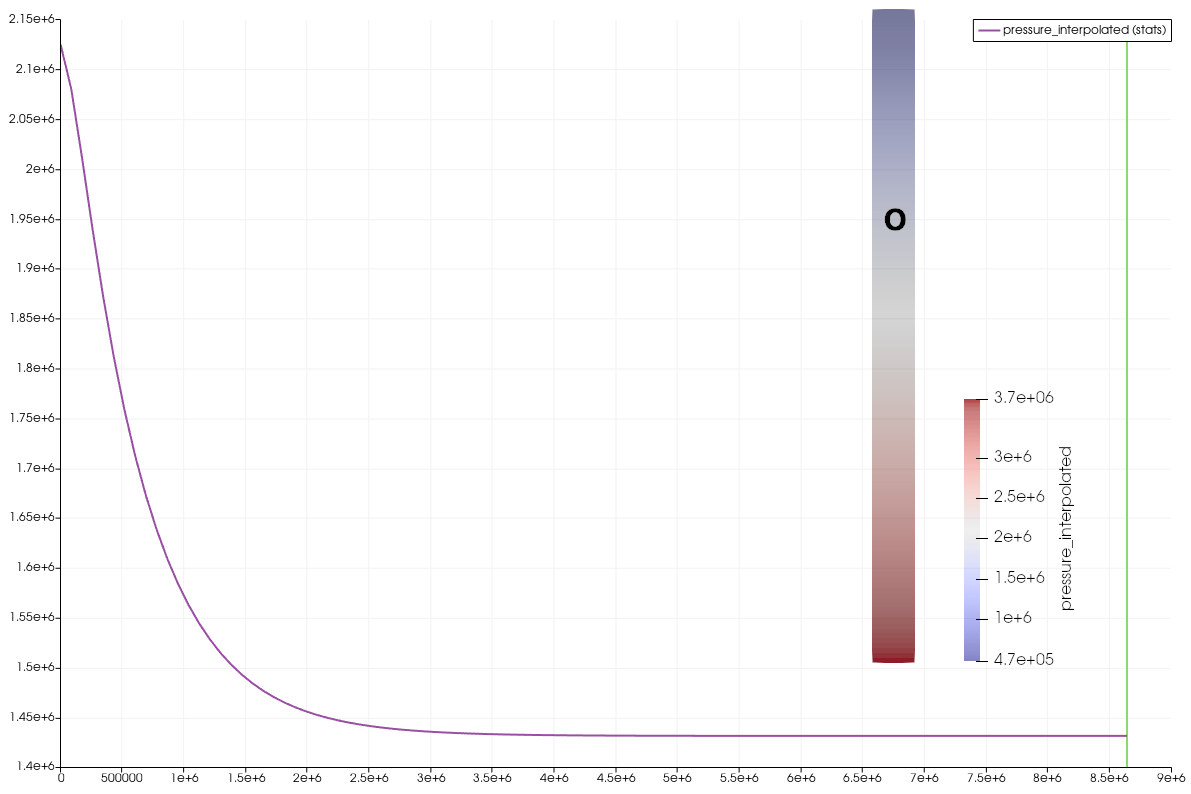
initial state	$p (x, y) = 2.125 \cdot 10^{6}$ Pa	$u_{x} (x, y) = u_{y} (x, y) = 0$

The gravity related terms are neglected in both: the Darcy velocity and the momentum balance equation.

Note that 100 time steps were used for the following results, whereas the provided input file is set to 1 time step (1 day = 86400 s). Kim plots his results over non dimensional time, referring to the time at which the produced fluid volume equals the pore volume of the domain (450 days).

Pressure at observation point (marked by circle) versus time (t=0…100 days) and spatial pressure distribution at t=100 days

Staggered Scheme: Fixed-stress splitting

For each time step run alternating simulations of the hydraulic (H) problem and the mechanical (M) problem until a convergence criteria is met. The fixed-stress split starts with the mass balance (H) followed by the momentum balance (M). These coupling iterations (H,M,H,M,…) add another iteration level compared to the monolithic formulation (HM). However, due to splitting into smaller problems this may result in a speedup.

The balance equations of mass and momentum for the fully saturated porous medium read

\begin{aligned} S ϱ_{f} \dot{p} - \frac{k}{μ} \nabla (ϱ_{f} (\nabla p - ϱ_{f} g)) + α ϱ_{f} {\dot{ε}}_{v} & = & 0 \\ \nabla \cdot (σ^{eff} (u) - α p I) & = & ϱ_{b} g . \end{aligned}

where $α$ denotes Biot coefficient, $S$ is the storage coefficient, $k$ is the intrinsic permeability, $μ$ the liquid viscosity, $ϱ_{f}$ is the fluid density, and $ϱ_{b}$ is the bulk density.

In the staggered scheme for solving HM coupled equations, the fixed-stress splitting is employed to enhance the convergence. The fixed stress splitting is based on the the volumetric total stress rate definition the hydro-mechanics:

{\dot{σ}}_{v} = K_{b} ({\dot{ε}}_{v} - {\dot{ε}}_{v}^{n e}) - α \dot{p},

with $K_{b}$ the drained bulk modulus of porous medium, and ${\dot{ε}}_{v}^{n e}$ the volumetric non-elastic strain rate.

Fixed stress rate over coupling iteration

As the first option, we consider to fix the volumetric total stress rate over coupling iteration. This means

{\dot{σ}}_{v}^{n, k} = {\dot{σ}}_{v}^{n, k - 1},

with $n$ the time step index, $k$ the coupling iteration index, and ${\dot{()}}^{n, k} = (()^{n, k} - ()^{n}) / d t$ .

This gives the volumetric strain rate of the current time step as

{\dot{ε_{v}}}^{n, k} \approx {\dot{ϵ}}_{v}^{n, k - 1} + \frac{α}{K_{b}} ({\dot{p}}^{n, k} - {\dot{p}}^{n, k - 1}) + ({\dot{ϵ}}_{v}^{n e} |^{n, k} - {\dot{ϵ}}_{v}^{n e} |^{n, k - 1}) .

Practically, we can set ${\dot{ϵ}}_{v}^{n e} |^{n, k} - {\dot{ϵ}}_{v}^{n e} |^{n, k - 1} = 0$ .

Under that volumetric strain rate approximation, the mass balance equation for coupling iteration $k$ at time step $n$ becomes

ϱ_{f} (β_{S} + \frac{α^{2}}{K_{b}}) {\dot{p}}^{n, k} - \frac{k}{μ} \nabla (ϱ_{f} (\nabla p^{n . k} - ϱ_{f} g)) + ϱ_{f} (α {\dot{ε}}_{v}^{n, k - 1} - \frac{α^{2}}{K_{b}} {\dot{p}}^{n, k - 1}) = 0.

Denoting $\frac{α^{2}}{K_{b}}$ as $β_{FS}$ , the above equation turns into

ϱ_{f} (β_{S} + β_{FS}) {\dot{p}}^{n, k} - \frac{k}{μ} \nabla (ϱ_{f} (\nabla p^{n . k} - ϱ_{f} g)) + ϱ_{f} (α {\dot{ε}}_{v}^{n, k - 1} - β_{FS} {\dot{p}}^{n, k - 1}) = 0.

One can see from the above equation that $β_{FS}$ can be any scalar number once the coupling iteration converges, i.e. ${\dot{p}}^{n, k} \approx {\dot{p}}^{n, k - 1}$ . Therefore, one can choose an arbitrary value for $β_{FS}$ if it can make the coupling iteration converge. The analysis by Mikelic and Wheeler [2] revealed that $β_{FS} = \frac{α^{2}}{2 K_{b}}$ is generally close to the a-priori unknown optimal value that enhances the convergence of the coupling iteration. For more information, see the user guide - conventions. For code implementation, we introduce a stabilization factor $γ$ to the physically meaningful parameter $\frac{α^{2}}{K_{b}}$ as:

β_{FS} = γ \frac{α^{2}}{K_{b}},

where $γ$ is treated as an input parameter.

Fixed stress rate over time step

We assume that the volumetric stress rate of the current time step is the same as that of the previous time step:

{\dot{σ}}_{v}^{n} = {\dot{σ}}_{v}^{n - 1} .

That means the current volumetric strain rate is approximated as

{\dot{ε_{v}}}^{n} \approx {\dot{ϵ}}_{v}^{n - 1} + \frac{α}{K_{b}} ({\dot{p}}^{n} - {\dot{p}}^{n - 1}) .

Consequently, and similarly to the fixed stress over coupling iteration, the mass balance equation at time step $n$ becomes

ϱ_{f} (S + β_{FS}) {\dot{p}}^{n} - \frac{k}{μ} \nabla (ϱ_{f} (\nabla p^{n} - ϱ_{f} g)) + ϱ_{f} (α {\dot{ε}}_{v}^{n - 1} - β_{FS} {\dot{p}}^{n - 1}) = 0.

In that sense, only one coupling iteration is needed, and the solution accuracy is dependent on the time step size. The approach of a fixed stress rate over the time step enables the staggered scheme to efficiently solve more HM problems, especially those with small strain change, e.g. hydro-mechanical modeling of reservoirs.

References

[1] Kim, J. and Tchelepi, H.A. and Juanes, R. (2009): Stability, Accuracy and Efficiency of Sequential Methods for Coupled Flow and Geomechanics. SPE International, vol. 16, p. 249--262, DOI:https://doi.org/10.2118/119084-PA https://onepetro.org/SJ/article-abstract/16/02/249/204235

[2] Mikelic, A. and Wheeler, M.F. (2013): Convergence of iterative coupling for coupled flow and geomechanics. Computational Geosciences, vol. 17, p. 455--461, DOI:https://doi.org/10.1007/s10596-012-9318-y https://link.springer.com/content/pdf/10.1007/s10596-012-9318-y.pdf

This article was written by Wenqing Wang and Dominik Kern. If you are missing something or you find an error please let us know.
Generated with Hugo 0.122.0 in CI job 545140 | Last revision: February 26, 2025
Commit: [PCS] Avoid to compute the analytic block in ed9789e | Edit this page on