Primary variable constraint Dirichlet-type boundary condition

• Parabolic/LiquidFlow/SimpleSynthetics/PrimaryVariableConstraintDirichletBC/cuboid_1x1x1_hex_1000_Dirichlet_Dirichlet_1.prj

Problem description

We start with the following parabolic PDE:

$$ \left( c \rho_R + \phi \frac{\partial \rho_R}{\partial p}\right) \frac{\partial p}{\partial t} - \nabla \cdot \left[ \rho_R \frac{\kappa}{\mu} \left( \nabla p + \rho_R g \right) \right] $$ $$ Q_p = 0. $$

where

• $c$ … a constant that characterizes the storage as a consequence that the solid phase is changing
• $\rho_R$ … the density
• $p$ … pressure
• $t$ … time
• $\kappa$ … the intrinsic permeability tensor of the porous medium
• $\mu$ … is the pressure dependent dynamic viscosity
• $Q_p$ … source/sink terms

In order to obtain a unique solution it is necessary to specify conditions on the boundary $\Gamma$ of the domain $\Omega$.

The benchmark at hand should demonstrate the primary variable constraint Dirichlet-type boundary condition. Here, the size of the sub-domain, the Dirichlet-type boundary condition is defined on, is variable and changes according to a condition depending on the value of the primary variable.

$$ \Gamma^\ast_D = \{ x \in \mathbb{R}^d, x \in \Gamma_D, \text{Condition}(p(x)) \} $$

Examples

On the left (x=0) and right side (x=1) of the domain $\Omega = [0,1]^3$ the usual Dirichlet-type boundary conditions are set, i.e.,

$$ p = 1, \quad x=0 \qquad \text{and} \qquad p = 1\quad x=1 $$

The initial condition $p_0$ is set to zero. Additionally, a primary variable constraint Dirichlet-type boundary condition (PVCDBC) is specified:

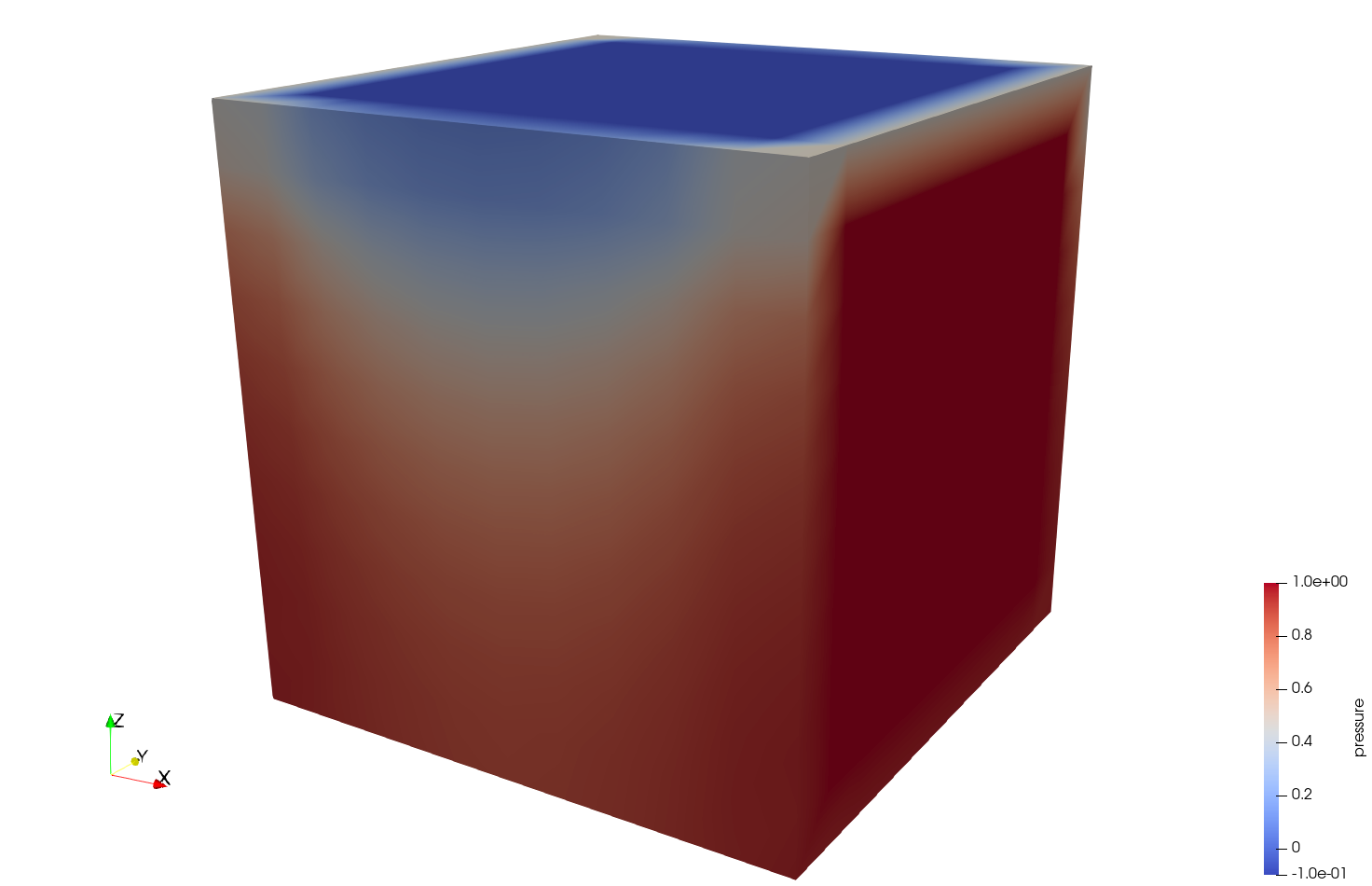
$$ p = -0.1, \quad \text{for}\quad z = 1 \quad \text{and}\quad p(x,y,1) > 0. $$

At the beginning of the simulation the PVCDBC is inactive. Because of the ’normal’ Dirichlet-type boundary conditions the pressure is greater than zero after the first time step and the PVCDBC is activated in the second time step. The effect is depicted in the figure: